
Gold Discovery Run, 2013
This spring I ran the Beat Beethoven 5K and had such a good time that I decided to give running another try. I’d tried adding running to my usual exercise routines in the past, but knee problems always sidelined me after a couple months. It’s been three months of slow increases in mileage using a marathon training plan by Hal Higdon, and so far so good.
My goal for this year, beyond staying healthy, is to participate in the 51st running of the Equinox Marathon here in Fairbanks.
One of the challenges for a beginning runner is how pace yourself during a race and how to know what your body can handle. Since Beat Beethoven I've run in the Lulu’s 10K, the Midnight Sun Run (another 10K), and last weekend I ran the 16.5 mile Gold Discovery Run from Cleary Summit down to Silver Gulch Brewery. I completed the race in two hours and twenty-nine minutes, at a pace of 9:02 minutes per mile. Based on this performance, I should be able to estimate my finish time and pace for Equinox by comparing the times for runners that participated in the 2012 Gold Discovery and Equinox.
The first challenge is extracting the data from the PDF files SportAlaska publishes after the race. I found that opening the PDF result files, selecting all the text on each page, and pasting it into a text file is the best way to preserve the formatting of each line. Then I process it through a Python function that extracts the bits I want:
import re
def parse_sportalaska(line):
    """ lines appear to contain:
        place, bib, name, town (sometimes missing), state (sometimes missing),
        birth_year, age_class, class_place, finish_time, off_win, pace,
        points (often missing) """
    fields = line.split()
    place = int(fields.pop(0))
    bib = int(fields.pop(0))
    name = fields.pop(0)
    while True:
        n = fields.pop(0)
        name = '{} {}'.format(name, n)
        if re.search('^[A-Z.-]+$', n):
            break
    pre_birth_year = []
    pre_birth_year.append(fields.pop(0))
    while True:
        try:
            f = fields.pop(0)
        except:
            print("Warning: couldn't parse: '{0}'".format(line.strip()))
            break
        else:
            if re.search('^[0-9]{4}$', f):
                birth_year = int(f)
                break
            else:
                pre_birth_year.append(f)
    if re.search('^[A-Z]{2}$', pre_birth_year[-1]):
        state = pre_birth_year[-1]
        town = ' '.join(pre_birth_year[:-1])
    else:
        state = None
        town = None
    try:
        (age_class, class_place, finish_time, off_win, pace) = fields[:5]
        class_place = int(class_place[1:-1])
        finish_minutes = time_to_min(finish_time)
        fpace = strpace_to_fpace(pace)
    except:
        print("Warning: couldn't parse: '{0}', skipping".format(
              line.strip()))
        return None
    else:
        return (place, bib, name, town, state, birth_year, age_class,
                class_place, finish_time, finish_minutes, off_win,
                pace, fpace)
The function uses a a couple helper functions that convert pace and time strings into floating point numbers, which are easier to analyze.
def strpace_to_fpace(p):
    """ Converts a MM:SS" pace to a float (minutes) """
    (mm, ss) = p.split(':')
    (mm, ss) = [int(x) for x in (mm, ss)]
    fpace = mm + (float(ss) / 60.0)

    return fpace

def time_to_min(t):
    """ Converts an HH:MM:SS time to a float (minutes) """
    (hh, mm, ss) = t.split(':')
    (hh, mm) = [int(x) for x in (hh, mm)]
    ss = float(ss)
    minutes = (hh * 60) + mm + (ss / 60.0)

    return minutes
Once I process the Gold Discovery and Equnox result files through this routine, I dump the results in a properly formatted comma-delimited file, read the data into R and combine the two race results files by matching the runner’s name. Note that these results only include the men competing in the race.
gd <- read.csv('gd_2012_men.csv', header=TRUE)
gd <- gd[,c('name', 'birth_year', 'finish_minutes', 'fpace')]
eq <- read.csv('eq_2012_men.csv', header=TRUE)
eq <- eq[,c('name', 'birth_year', 'finish_minutes', 'fpace')]
combined <- merge(gd, eq, by='name')
names(combined) <- c('name', 'birth_year', 'gd_finish', 'gd_pace',
                     'year', 'eq_finish', 'eq_pace')
When I look at a plot of the data I can see four outliers; two where the runners ran Equinox much faster based on their Gold Discovery pace, and two where the opposite was the case. The two races are two months apart, so I think it’s reasonable to exclude these four rows from the data since all manner of things could happen to a runner in two months of hard training (or on race day!).
attach(combined)
combined <- combined[!((gd_pace > 10 & gd_pace < 11 & eq_pace > 15)
                       | (gd_pace > 15)),]
Let’s test the hypothesis that we can predict Equinox pace from Gold Discovery Pace:
model <- lm(eq_pace ~ birth_year, data=combined)
summary(model)

Call:
lm(formula = eq_pace ~ gd_pace, data = combined)

Residuals:
     Min       1Q   Median       3Q      Max
-1.47121 -0.36833 -0.04207  0.51361  1.42971

Coefficients:
            Estimate Std. Error t value Pr(>|t|)
(Intercept)  0.77392    0.52233   1.482    0.145
gd_pace      1.08880    0.05433  20.042   <2e-16 ***
---
Signif. codes:  0 ‘***’ 0.001 ‘**’ 0.01 ‘*’ 0.05 ‘.’ 0.1 ‘ ’ 1

Residual standard error: 0.6503 on 48 degrees of freedom
Multiple R-squared:  0.8933,    Adjusted R-squared:  0.891
F-statistic: 401.7 on 1 and 48 DF,  p-value: < 2.2e-16
Indeed, we can explain 65% of the variation in Equinox Marathon pace times using Gold Discovery pace times, and both the model and the model coefficient are significant.
Here’s what the results look like:
The red line shows a relationship where the Gold Discovery pace is identical to the Equinox pace for each running. Because the actual data (and the prediced results based on the regression model) are above this line, that means that all the runners were slower in the longer (and harder) Equinox Marathon.
As for me, my 9:02 Gold Discovery pace should translate into an Equinox pace around 10:30. Here are the 2012 runners who were born within ten years of me, and who finished within ten minutes of my 2013 Gold Discovery time:
| Runner | DOB | Gold Discovery | Equinox Time | Equinox Pace |
|---|---|---|---|---|
| Dan Bross | 1964 | 2:24 | 4:20 | 9:55 |
| Chris Hartman | 1969 | 2:25 | 4:45 | 10:53 |
| Mike Hayes | 1972 | 2:27 | 4:58 | 11:22 |
| Ben Roth | 1968 | 2:28 | 4:47 | 10:57 |
| Jim Brader | 1965 | 2:31 | 4:09 | 9:30 |
| Erik Anderson | 1971 | 2:32 | 5:03 | 11:34 |
| John Scherzer | 1972 | 2:33 | 4:49 | 11:01 |
| Trent Hubbard | 1972 | 2:33 | 4:48 | 11:00 |
Based on this, and the regression results, I expect to finish the Equinox Marathon in just under five hours if my training over the next two months goes well.
Cold November
Several years ago I showed some R code to make a heatmap showing the rank of the Oakland A’s players for various hitting and pitching statistics.
Last week I used this same style of plot to make a new weather visualization on my web site: a calendar heatmap of the difference between daily average temperature and the “climate normal” daily temperature for all dates in the last ten years. “Climate normals” are generated every ten years and are the averages for a variety of statistics for the previous 30-year period, currently 1981—2010.
A calendar heatmap looks like a normal calendar, except that each date box is colored according to the statistic of interest, in this case the difference in temperature between the temperature on that date and the climate normal temperature for that date. I also created a normalized version based on the standard deviations of temperature on each date.
Here’s the temperature anomaly plot showing all the temperature differences for the last ten years:
It’s a pretty incredible way to look at a lot of data at the same time, and it makes it really easy to pick out anomalous events such as the cold November and December of 2012. One thing you can see in this plot is that the more dramatic temperature differences are always in the winter; summer anomalies are generally smaller. This is because the range of likely temperatures is much larger in winter, and in order to equalize that difference, we need to normalize the anomalies by this range.
One way to do that is to divide the actual temperature difference by the standard deviation of the 30-year climate normal mean temperature. Because of the nature of the distribution standard deviations are based on, approximately 66% of the variation occurrs within -1 and 1 standard deviation, 95% between -2 and 2, and 99% between -3 and 3 standard deviations. That means that deep red or blue dates, those outside of -3 and 3, in the normalized calendar plot are fairly rare occurrances.
Here’s the normalized anomalies for the last twelve months:
The tricky part in generating either of these plots is getting the temperature data into the right format. The plots are faceted by month and year (or YYYYY-MM in the twelve month plot), so each record needs to have month and year. That part is easy. Each individual plot is a single calendar month, and is organized by day of the week along the x-axis, and the inverse of week number along the y-axis (the first week in a month is at the top of the plot, the last at the bottom).
Here’s how to get the data formatted properly:
library(lubridate)
cal <- function(dt) {
    # Reads a date object and returns a tuple (weekrow, daycol)
    # where weekrow starts at 1 and daycol starts at 1 for Sunday
    year <- year(dt)
    month <- month(dt)
    day <- day(dt)
    wday_first <- wday(ymd(paste(year, month, 1, sep = '-'), quiet = TRUE))
    offset <- 7 + (wday_first - 2)
    weekrow <- ((day + offset) %/% 7) - 1
    daycol <- (day + offset) %% 7

    c(weekrow, daycol)
}
weekrow <- function(dt) {
    cal(dt)[1]
}
daycol <- function(dt) {
    cal(dt)[2]
}
vweekrow <- function(dts) {
    sapply(dts, weekrow)
}
vdaycol <- function(dts) {
    sapply(dts, daycol)
}
pafg$temp_anomaly <- pafg$mean_temp - pafg$average_mean_temp
pafg$month <- month(pafg$dt, label = TRUE, abbr = TRUE)
pafg$year <- year(pafg$dt)
pafg$weekrow <- factor(vweekrow(pafg$dt),
   levels = c(5, 4, 3, 2, 1, 0),
   labels = c('6', '5', '4', '3', '2', '1'))
pafg$daycol <- factor(vdaycol(pafg$dt),
   labels = c('u', 'm', 't', 'w', 'r', 'f', 's'))
And the plotting code:
library(ggplot2)
library(scales)
library(grid)
svg('temp_anomaly_heatmap.svg', width = 11, height = 10)
q <- ggplot(data = subset(pafg, year > max(pafg$year) - 11),
            aes(x = daycol, y = weekrow, fill = temp_anomaly)) +
    theme_bw() +
    theme(axis.text.x = element_blank(),
          axis.text.y = element_blank(),
          panel.grid.major = element_blank(),
          panel.grid.minor = element_blank(),
          axis.ticks.x = element_blank(),
          axis.ticks.y = element_blank(),
          axis.title.x = element_blank(),
          axis.title.y = element_blank(),
          legend.position = "bottom",
          legend.key.width = unit(1, "in"),
          legend.margin = unit(0, "in")) +
    geom_tile(colour = "white") +
    facet_grid(year ~ month) +
    scale_fill_gradient2(name = "Temperature anomaly (°F)",
          low = 'blue', mid = 'lightyellow', high = 'red',
          breaks = pretty_breaks(n = 10)) +
    ggtitle("Difference between daily mean temperature\
             and 30-year average mean temperature")
print(q)
dev.off()
You can find the current versions of the temperature and normalized anomaly plots at:
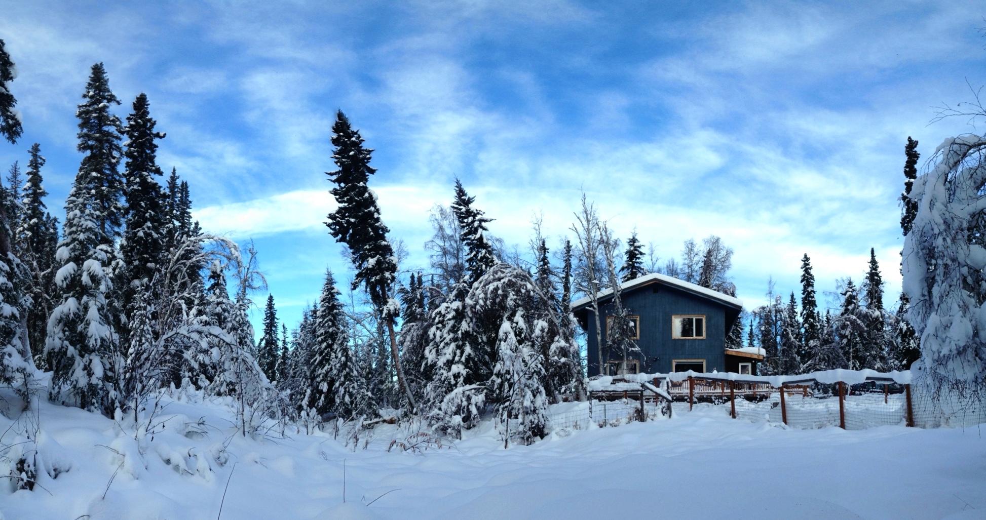
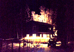
House from the slough
A couple days ago I got an email from a Galoot who was hoping to come north to see the aurora and wondered if March was a good time to come to Fairbanks. I know that March and September are two of my favorite months, but wanted to check to see if my perception of how sunny it is in March was because it really is sunny in March or if it’s because March is the month when winter begins to turn to spring in Fairbanks and it just seems brighter and sunnier, with longer days and white snow on the ground.
I found three sources of data for “cloudiness.” I’ve been parsing the Fairbanks Airport daily climate summary since 2002, and it has a value in it called Average Sky Cover which ranges from 0.0 (completely clear) to 1.0 (completely cloudy). I’ll call this data “pafa.”
The second source is the Global Historical Climatology - Daily for the Fairbanks Airport station. There’s a variable in there named ACMH, which is described as Cloudiness, midnight to midnight (percentage). For the Airport station, this value appears in the database from 1965 through 1997. One reassuring thing about this parameter is that it specifically says it’s from midnight to midnight, so it would include cloudiness when it was dark outside (and the aurora would be visible if it was present). This data set is named “ghcnd.”
The final source is modelled data from the North American Regional Reanalysis. This data set includes TCDC, or total cloud cover (percentage), and is available in three-hour increments over a grid covering North America. I chose the nearest grid point to the Fairbanks Airport and retrieved the daily mean of total cloud cover for the period of the database I have downloaded (1979—2012). In the plots that follow, this is named “narr.”
After reading the data and merging the three data sets together, I generate monthly means of cloud cover (scaled to percentages from 0 to 100) in each of the data sets, in R:
library(plyr)
cloud_cover <- merge(pafa, ghcnd, by = 'date', all = TRUE)
cloud_cover <- merge(cloud_cover, narr, by = 'date', all = TRUE)
cloud_cover$month <- month(cloud_cover$date)

by_month_mean <- ddply(
    subset(cloud_cover,
           select = c('month', 'pafa', 'ghcnd', 'narr')),
   .(month),
   summarise,
   pafa = mean(pafa, na.rm = TRUE),
   ghcnd = mean(ghcnd, na.rm = TRUE),
   narr = mean(narr, na.rm = TRUE))
by_month_mean$mon <- factor(by_month_mean$month,
                            labels = c('jan', 'feb', 'mar',
                                       'apr', 'may', 'jun',
                                       'jul', 'aug', 'sep',
                                       'oct', 'nov', 'dec'))
In order to plot it, I generate text labels for the year range of each data set and melt the data so it can be faceted:
library(lubridate)
library(reshape2)
text_labels <- rbind(
    data.frame(variable = 'pafa',
        str = paste(min(year(pafa$date)), '-', max(year(pafa$date)))),
    data.frame(variable = 'ghcnd',
        str = paste(min(year(ghcnd$date)), '-', max(year(ghcnd$date)))),
    data.frame(variable = 'narr',
        str = paste(min(year(narr$date)), '-', max(year(narr$date)))))

mean_melted <- melt(by_month_mean,
                    id.vars = 'mon',
                    measure.vars = c('pafa', 'ghcnd', 'narr'))
Finally, the plotting:
library(ggplot2)
q <- ggplot(data = mean_melted, aes(x = mon, y = value))
q +
    theme_bw() +
    geom_bar(stat = 'identity', colour = "darkred", fill = "darkorange") +
    facet_wrap(~ variable, ncol = 1) +
    scale_x_discrete(name = "Month") +
    scale_y_continuous(name = "Mean cloud cover") +
    ggtitle('Cloud cover data for Fairbanks Airport Station') +
    geom_text(data = text_labels, aes(x = 'feb', y = 70, label = str), size = 4) +
    geom_text(aes(label = round(value, digits = 1)), vjust = 1.5, size = 3)
The good news for the guy coming to see the northern lights is that March is indeed the least cloudy month in Fairbanks, and all three data sources show similar patterns, although the NARR dataset has September and October as the cloudiest months, and anyone who has lived in Fairbanks knows that August is the rainiest (and probably cloudiest) month. PAFA and GHCND have a late summer pattern that seems more like what I recall.
Another way to slice the data is to get the average number of days in a month with less than 20% cloud cover; a measure of the clearest days. This is a pretty easy calculation:
by_month_less_than_20 <- ddply(
    subset(cloud_cover,
           select = c('month', 'pafa', 'ghcnd', 'narr')),
    .(month),
    summarise,
    pafa = sum(pafa < 20, na.rm = TRUE) / sum(!is.na(pafa)) * 100,
    ghcnd = sum(ghcnd < 20, na.rm = TRUE) / sum(!is.na(ghcnd)) * 100,
    narr = sum(narr < 20, na.rm = TRUE) / sum(!is.na(narr)) * 100);
And the results:
We see the same pattern as in the mean cloudiness plot. March is the month with the greatest number of days with less that 20% cloud cover. Depending on the data set, between 17 and 24 percent of March days are quite clear. In contrast, the summer months rarely see days with no cloud cover. In June and July, the days are long and convection often builds large clouds in the late afternoon, and by August, the rain has started. Just like in the previous plot, NARR has September as the month with the fewest clear days, which doesn’t match my experience.
It’s now December 1st and the last time we got new snow was on November 11th. In my last post I looked at the lengths of snow-free periods in the available weather data for Fairbanks, now at 20 days. That’s a long time, but what I’m interested in looking at today is whether the monthly pattern of snowfall in Fairbanks is changing.
The Alaska Dog Musher’s Association holds a series of weekly sprint races starting at the beginning of December. For the past several years—and this year—there hasn’t been enough snow to hold the earliest of the races because it takes a certain depth of snowpack to allow a snow hook to hold a team back should the driver need to stop. I’m curious to know if scheduling a bunch of races in December and early January is wishful thinking, or if we used to get a lot of snow earlier in the season than we do now. In other words, has the pattern of snowfall in Fairbanks changed?
One way to get at this is to look at the earliest data in the “winter year” (which I’m defining as starting on September 1st, since we do sometimes get significant snowfall in September) when 12 inches of snow has fallen. Here’s what that relationship looks like:
And the results from a linear regression:
Call:
lm(formula = winter_doy ~ winter_year, data = first_foot)

Residuals:
    Min      1Q  Median      3Q     Max
-60.676 -25.149  -0.596  20.984  77.152

Coefficients:
             Estimate Std. Error t value Pr(>|t|)
(Intercept) -498.5005   462.7571  -1.077    0.286
winter_year    0.3067     0.2336   1.313    0.194

Residual standard error: 33.81 on 60 degrees of freedom
Multiple R-squared: 0.02793,    Adjusted R-squared: 0.01173
F-statistic: 1.724 on 1 and 60 DF,  p-value: 0.1942
According to these results the date of the first foot of snow is getting later in the year, but it’s not significant, so we can’t say with any authority that the pattern we see isn’t just random. Worse, this analysis could be confounded by what appears to be a decline in the total yearly snowfall in Fairbanks:
This relationship (less snow every year) has even less statistical significance. If we combine the two analyses, however, there is a significant relationship:
Call:
lm(formula = winter_year ~ winter_doy * snow, data = yearly_data)

Residuals:
   Min     1Q Median     3Q    Max
-35.15 -11.78   0.49  14.15  32.13

Coefficients:
                  Estimate Std. Error t value Pr(>|t|)
(Intercept)      1.947e+03  2.082e+01  93.520   <2e-16 ***
winter_doy       4.297e-01  1.869e-01   2.299   0.0251 *
snow             5.248e-01  2.877e-01   1.824   0.0733 .
winter_doy:snow -7.022e-03  3.184e-03  -2.206   0.0314 *
---
Signif. codes:  0 ‘***’ 0.001 ‘**’ 0.01 ‘*’ 0.05 ‘.’ 0.1 ‘ ’ 1

Residual standard error: 17.95 on 58 degrees of freedom
Multiple R-squared: 0.1078,     Adjusted R-squared: 0.06163
F-statistic: 2.336 on 3 and 58 DF,  p-value: 0.08317
Here we’re “predicting” winter year based on the yearly snowfall, the first date where a foot of snow had fallen, and the interaction between the two. Despite the near-significance of the model and the parameters, it doesn’t do a very good job of explaining the data (almost 90% of the variation is unexplained by this model).
One problem with boiling the data down into a single (or two) values for each year is that we’re reducing the amount of data being analyzed, lowering our power to detect a significant relationship between the pattern of snowfall and year. Here’s what the overall pattern for all years looks like:
And the individual plots for each year in the record:
Because “winter month” isn’t a continuous variable, we can’t use normal linear regression to evaluate the relationship between year and monthly snowfall. Instead we’ll use multinominal logistic regression to investigate the relationship between which month is the snowiest, and year:
library(nnet)
model <- multinom(data = snowiest_month, winter_month ~ winter_year)
summary(model)

Call:
multinom(formula = winter_month ~ winter_year, data = snowiest_month)

Coefficients:
  (Intercept)  winter_year
3    30.66572 -0.015149192
4    62.88013 -0.031771508
5    38.97096 -0.019623059
6    13.66039 -0.006941225
7   -68.88398  0.034023510
8   -79.64274  0.039217108

Std. Errors:
   (Intercept)  winter_year
3 9.992962e-08 0.0001979617
4 1.158940e-07 0.0002289479
5 1.120780e-07 0.0002218092
6 1.170249e-07 0.0002320081
7 1.668613e-07 0.0003326432
8 1.955969e-07 0.0003901701

Residual Deviance: 221.5413
AIC: 245.5413
I’m not exactly sure how to interpret the results, but typically you’re looking to see if the intercepts and coefficients are significantly different from zero. If you look at the difference in magnitude between the coefficients and the standard errors, it appears they are significantly different from zero, which would imply they are statistically significant.
In order to examine what they have to say, we’ll calculate the probability curves for whether each month will wind up as the snowiest month, and plot the results by year.
fit_snowiest <- data.frame(winter_year = 1949:2012)
probs <- cbind(fit_snowiest, predict(model, newdata = fit_snowiest, "probs"))
probs.melted <- melt(probs, id.vars = 'winter_year')
names(probs.melted) <- c('winter_year', 'winter_month', 'probability')
probs.melted$month <- factor(probs.melted$winter_month)
levels(probs.melted$month) <- \
  list('oct' = 2, 'nov' = 3, 'dec' = 4, 'jan' = 5, 'feb' = 6, 'mar' = 7, 'apr' = 8)
q <- ggplot(data = probs.melted, aes(x = winter_year, y = probability, colour = month))
q + theme_bw() + geom_line(size = 1) + scale_y_continuous(name = "Model probability") \
  + scale_x_continuous(name = 'Winter year', breaks = seq(1945, 2015, 5)) \
  + ggtitle('Snowiest month probabilities by year from logistic regression model,\n
    Fairbanks Airport station') \
  + scale_colour_manual(values = \
    c("violet", "blue", "cyan", "green", "#FFCC00", "orange", "red"))
The result:
Here’s how you interpret this graph. Each line shows how likely it is that a month will be the snowiest month (November is always the snowiest month because it always has the highest probabilities). The order of the lines for any year indicates the monthly order of snowiness (in 1950, November, December and January were predicted to be the snowiest months, in that order), and months with a negative slope are getting less snowy overall (November, December, January).
November is the snowiest month for all years, but it’s declining, as is snow in December and January. October, February, March and April are increasing. From these results, it appears that we’re getting more snow at the very beginning (October) and at the end of the winter, and less in the middle of the winter.
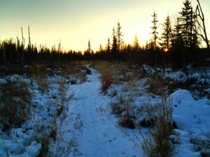
Early-season ski from work
Yesterday a co-worker and I were talking about how we weren’t able to enjoy the new snow because the weather had turned cold as soon as the snow stopped falling. Along the way, she mentioned that it seemed to her that the really cold winter weather was coming later and later each year. She mentioned years past when it was bitter cold by Halloween.
The first question to ask before trying to determine if there has been a change in the date of the first cold snap is what qualifies as “cold.” My officemate said that she and her friends had a contest to guess the first date when the temperature didn’t rise above -20°F. So I started there, looking for the month and day of the winter when the maximum daily temperature was below -20°F.
I’m using the GHCN-Daily dataset from NCDC, which includes daily minimum and maximum temperatures, along with other variables collected at each station in the database.
When I brought in the data for the Fairbanks Airport, which has data available from 1948 to the present, there was absolutely no relationship between the first -20°F or colder daily maximum and year.
However, when I changed the definition of “cold” to the first date when the daily minimum temperature is below -40, I got a weak (but not statistically significant) positive trend between date and year.
The SQL query looks like this:
SELECT year, water_year, water_doy, mmdd, temp
FROM (
    SELECT year, water_year, water_doy, mmdd, temp,
        row_number() OVER (PARTITION BY water_year ORDER BY water_doy) AS rank
    FROM (
        SELECT extract(year from dte) AS year,
            extract(year from dte + interval '92 days') AS water_year,
            extract(doy from dte + interval '92 days') AS water_doy,
            to_char(dte, 'mm-dd') AS mmdd,
            sum(CASE WHEN variable = 'TMIN'
                     THEN raw_value * raw_multiplier
                     ELSE NULL END
               ) AS temp
        FROM ghcnd_obs
            INNER JOIN ghcnd_variables USING(variable)
        WHERE station_id = 'USW00026411'
        GROUP BY extract(year from dte),
            extract(year from dte + interval '92 days'),
            extract(doy from dte + interval '92 days'),
            to_char(dte, 'mm-dd')
        ORDER BY water_year, water_doy
    ) AS foo
    WHERE temp < -40 AND temp > -80
) AS bar
WHERE rank = 1
ORDER BY water_year;
I used “water year” instead of the actual year because the winter is split between two years. The water year starts on October 1st (we’re in the 2013 water year right now, for example), which converts a split winter (winter of 2012/2013) into a single year (2013, in this case). To get the water year, you add 92 days (the sum of the days in October, November and December) to the date and use that as the year.
Here’s what it looks like (click on the image to view a PDF version):
The dots are the observed date of first -40° daily minimum temperature for each water year, and the blue line shows a linear regression model fitted to the data (with 95% confidence intervals in grey). Despite the scatter, you can see a slightly positive slope, which would indicate that colder temperatures in Fairbanks are coming later now, than they were in the past.
As mentioned, however, our eyes often deceive us, so we need to look at the regression model to see if the visible relationship is significant. Here’s the R lm results:
Call:
lm(formula = water_doy ~ water_year, data = first_cold)

Residuals:
    Min      1Q  Median      3Q     Max
-45.264 -15.147  -1.409  13.387  70.282

Coefficients:
             Estimate Std. Error t value Pr(>|t|)
(Intercept) -365.3713   330.4598  -1.106    0.274
water_year     0.2270     0.1669   1.360    0.180

Residual standard error: 23.7 on 54 degrees of freedom
Multiple R-squared: 0.0331,     Adjusted R-squared: 0.01519
F-statistic: 1.848 on 1 and 54 DF,  p-value: 0.1796
The first thing to check in the model summary is the p-value for the entire model on the last line of the results. It’s only 0.1796, which means that there’s an 18% chance of getting these results simply by chance. Typically, we’d like this to be below 5% before we’d consider the model to be valid.
You’ll also notice that the coefficient of the independent variable (water_year) is positive (0.2270), which means the model predicts that the earliest cold snap is 0.2 days later every year, but that this value is not significantly different from zero (a p-value of 0.180).
Still, this seems like a relationship worth watching and investigating further. It might be interesting to look at other definitions of “cold,” such as requiring three (or more) consecutive days of -40° temperatures before including that period as the earliest cold snap. I have a sense that this might reduce the year to year variation in the date seen with the definition used here.