Over the past couple weeks I’ve been experimenting with a data logging shield from adafruit. My original idea was to build a unit I could take with my on my commute to work to see how the temperatures change over the route. I’m also interested in watching the temperatures inside a dog house when there’s a dog sleeping in there. During the cold snap, where temperatures got as low as -55°F, how warm could the dogs keep their houses (which are insulated)?
I added a three axis accelerometer (ADXL335) with the idea it could tell me when I was moving, but I don’t think I can afford to read (and log) the sensors that often when it’s running off batteries (6 AA cells) at cold temperature. Instead, it’ll tell me the position (relative to the ground) of the logger, and I’ll use that to indicate when I start whatever activity I want to measure. The data logger starts logging as soon as it gets power, and even though it has a clock, it may drift relative to GPS time, so I can time the start based on when the logger’s position changes.
Here’s the schematic:
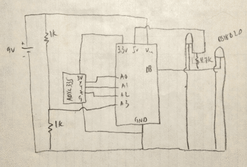
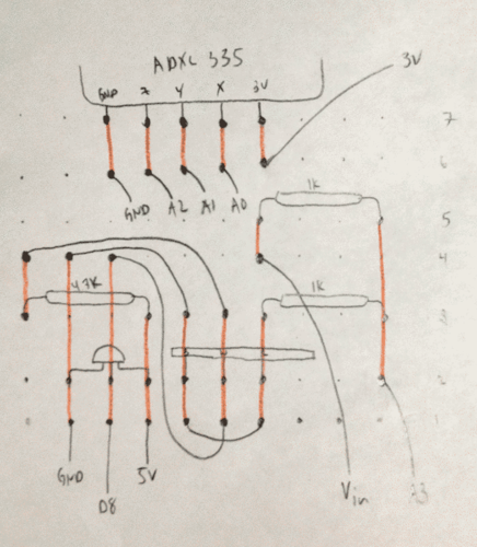
I wired it on a breadboard first to confirm the circuit was correct and to get the program storing the data. The data logger shield has a 10 x 10 perfboard section, so once everything was working, I soldered the parts directly onto the board using the plan below. The black lines are above the board and the orange lines are the solder joins below the board.
I don’t know yet how long the battery will last, but I ran it last night in the arctic entryway and got the following data:
The orange dots are from the temperature sensor on the board, wrapped in bubble wrap and sitting inside a cardboard box. The cyan dots are from the waterproof sensor outside of the box. Our arctic entryway is heated with a ventilation fan that blows warm air from the house into the room, so the oscillation in the temperature shows the fan going on at the bottom of the sweep and then off at the top. The insulation in the box reduces the temperature fluctuations and traps the slight amount of heat produced by the electronics.
Time to watch the Super Bowl.
In my last post I discussed the January 2012 cold snap, which was the fifth coldest January on record in Fairbanks. I wondered how much of this was due to the arbitrary choice of “month” as the aggregation level for the analysis. In other words, maybe January 2012 was really remarkable only because the cold happened to fall within the margins of that particular month?
So I ran a query against the GHCN daily database for the Fairbanks Airport station. This data set won’t allow me to answer the exact question I’m interested in because the data for Fairbanks only goes back to 1948 and because I don’t have the data for the last day in January 2012. But I think the analysis is still valid, even if it’s not perfect.
The following query calculates the average temperature in Fairbanks for every 31-day period possible, and ranks it according to a descending sort of the average temperature for those periods. The results show the start date, end date, the year and month that the majority of data appears in (more on that later), and the average temperature over the period.
One other note: the temperatures in this post are in degrees Celsius, which is why they’re different than those in my previous post (in °F).
SELECT date(dte - interval '15 days') AS start,
       date(dte + interval '15 days') AS end,
       to_char(dte, 'YYYY-MM') AS yyyymm,
       round(avg_31_days::numeric, 1),
       rank() OVER (ORDER BY avg_31_days) AS rank
FROM (
    SELECT dte,
           avg(tavg_c) OVER (
              ORDER BY dte
              ROWS BETWEEN 15 PRECEDING AND 15 FOLLOWING
           ) AS avg_31_days
    FROM (
        SELECT dte,
               (sum(CASE WHEN variable = 'TMIN'
                    THEN raw_value * 0.1
                    ELSE NULL END)
              + sum(CASE WHEN variable = 'TMAX'
                    THEN raw_value * 0.1
                    ELSE NULL END)) / 2.0 AS tavg_c
        FROM ghcnd_obs
        WHERE station_id = 'USW00026411'
        GROUP BY dte
    ) AS foo
) AS bar
ORDER BY rank;
The funky CASE WHEN ... END stuff in the innermost query is because of the structure of the data in the GHCN database. The exciting part is the window function in the first subquery that calculates the average temperature for a 31-day window surrounding every date in the database.
Some of the results:
| start | end | yyyymm | avg (°C) | rank |
|---|---|---|---|---|
| 1964-12-10 | 1965-01-09 | 1964-12 | -36.9 | 1 |
| 1964-12-09 | 1965-01-08 | 1964-12 | -36.9 | 2 |
| 1964-12-11 | 1965-01-10 | 1964-12 | -36.9 | 2 |
| 1971-01-06 | 1971-02-05 | 1971-01 | -36.8 | 4 |
| 1964-12-08 | 1965-01-07 | 1964-12 | -36.7 | 5 |
| 1971-01-07 | 1971-02-06 | 1971-01 | -36.6 | 6 |
| 1971-01-05 | 1971-02-04 | 1971-01 | -36.5 | 7 |
| 1964-12-12 | 1965-01-11 | 1964-12 | -36.4 | 8 |
| 1968-12-21 | 1969-01-20 | 1969-01 | -36.3 | 9 |
| 1968-12-22 | 1969-01-21 | 1969-01 | -36.3 | 10 |
| ... | ||||
| 2012-01-14 | 2012-02-13 | 2012-01 | -33.9 | 42 |
| 2012-01-13 | 2012-02-12 | 2012-01 | -33.9 | 43 |
There are some interesting things here. First, the January we just went through doesn’t show up until the 42nd coldest. You can also see that there was a very cold period from mid-December 1964 through mid-January 1964. This “even” appears five times in the first ten coldest periods. The January 1971 event occurs three times in the top ten.
To me, this means a couple things. First, we’re diluting the rankings because the same cold weather event shows up multiple times. If we use the yyyymm column to combine these, we can get a better sense of where January 2012 fits. Also, if an event shows up on here a bunch of times, that probably means that the event was longer than the 31-day window we’ve set at the outset. If you look at the minimum and maximum dates for the 1964 event, the real even lasted from December 8, 1964 through January 11, 1964 (35 days).
If we use this query as a subquery of one that groups on yyyymm, we’ll get a ranking of the overall events:
SELECT yyyymm, min_avg,
       rank() OVER (ORDER BY min_rank)
FROM (
    SELECT yyyymm,
           min(avg_31_days) AS min_avg,
           min(rank) AS min_rank
    FROM (ABOVE QUERY) AS foobie
    GROUP BY yyyymm
) AS barfoo
ORDER BY min_rank;
Here’s the results of the new query:
| yyyymm | min_avg (°C) | rank |
|---|---|---|
| 1964-12 | -36.9 | 1 |
| 1971-01 | -36.8 | 2 |
| 1969-01 | -36.3 | 3 |
| 1951-01 | -34.2 | 4 |
| 1996-11 | -34.0 | 5 |
| 2012-01 | -33.9 | 6 |
| 1953-01 | -33.7 | 7 |
| 1956-12 | -33.5 | 8 |
| 1966-01 | -33.3 | 9 |
| 1965-01 | -33.2 | 10 |
Our cold snap winds up in sixth place. I’m sure that if I had all the data the National Weather Service used in their analysis, last month would drop even lower in an analysis like this one.
My conclusion: last month was a really cold month. But the exceptional nature of it was at least partly due to the coincidence of it happening within the confines of an arbitrary 31-day period called “January.”
January 2012 was a historically cold month in Fairbanks, the fifth-coldest in more than 100 years of records. According to the National Weather Service office in Fairbanks:
January 2012 was the coldest month in more than 40 years in Fairbanks. Not since January 1971 has the Fairbanks area endured a month as cold as this.
The average high temperature for January was 18.2 below and the average low was 35 below. The monthly average temperature of 26.9 below was 19 degrees below normal and made this the fifth coldest January of record. The coldest January of record was 1971, when the average temperature was 31.7 below. The highest temperature at the airport was 21 degrees on the 10th, one of only three days when the temperature rose above zero. This ties with 1966 as the most days in January with highs of zero or lower. There were 16 days with a low temperature of 40 below or lower. Only four months in Fairbanks in more than a century of weather records have had more 40 below days. The lowest temperature at the airport was 51 below on the 29th.
Here’s a figure showing some of the relevant information:
The vertical bars show how much colder (or warmer for the red bars) the average daily temperature at the airport was compared with the 30-year average. You can see from these bars that we had only four days where the temperature was slightly above normal. The blue horizontal line shows the average anomaly for the period, and the orange (Fairbanks airport) and dark cyan (Goldstream Creek) horizontal lines show the actual average temperatures over the period. The average temperature at our house was -27.7°F for the month of January.
Finally, the circles and + symbols represent the minimum daily temperatures recorded at the airport (orange) and our house (dark cyan). You can see the two days late in the month where we got down to -54 and -55°F; cold enough that the propane in our tank remained a liquid and we couldn’t use our stove without heating up the tank.
No matter how you slice it, it was a very cold month.
Here’s some of the R code used to make the plot:
library(lubridate)
library(ggplot2)
library(RPostgreSQL)
# (Read in dw1454 data here)
dw_1454$date <- force_tz(
    ymd(as.character(dw_1454$date)),
    tzone = "America/Anchorage")
dw_1454$label <- 'dw1454 average'
# (Read FAI data here)
plot_data$line_color <- as.factor(
    as.numeric(plot_data$avg_temp_anomaly > 0))
plot_data$anomaly <- as.factor(
    ifelse(plot_data$line_color == 0,
        "degrees colder",
        "degrees warmer"))
plot_data$daily <- 'FAI average'

q <- ggplot(data = plot_data,
    aes(x = date + hours(9))) # TZ?
q + geom_hline(y = avg_mean_anomaly,
        colour = "blue", size = 0.25) +
    geom_hline(y = avg_mean_pafg,
        colour = "orange", size = 0.25) +
    geom_hline(y = avg_mean_dw1454,
        colour = "darkcyan", size = 0.25) +
    geom_linerange(aes(ymin = avg_temp_anomaly,
        ymax = 0, colour = anomaly)) +
    theme_bw() +
    scale_y_continuous(name = "Temperature (degrees F)") +
    scale_color_manual(name = "Daily temperature",
        c("degrees colder" = "blue",
          "degrees warmer" = "red",
          "FAI average" = "orange",
          "dw1454 average" = "darkcyan")) +
    scale_x_datetime(name = "Date") +
    geom_point(aes(y = min_temp,
        colour = daily), shape = 1, size = 1) +
    geom_point(data = dw_1454,
        aes(x = date, y = dw1454_min,
            colour = label), shape = 3, size = 1) +
    opts(title = "Average Daily Temperature Anomaly") +
    geom_text(aes(x = ymd('2012-01-31'),
        y = avg_mean_dw1454 - 1.5),
        label = round(avg_mean_dw1454, 1),
        colour = "darkcyan", size = 4)

Skiing at -34
This morning I skied to work at the coldest temperatures I’ve ever attempted (-31°F when I left). We also got more than an inch of snow yesterday, so not only was it cold, but I was skiing in fresh snow. It was the slowest 4.1 miles I’d ever skied to work (57+ minutes!) and as I was going, I thought about what factors might explain how fast I ski to and from work.
Time to fire up R and run some PostgreSQL queries. The first query grabs the skiing data for this winter:
SELECT start_time,
    (extract(epoch from start_time) - extract(epoch from '2011-10-01':date))
        / (24 * 60 * 60) AS season_days,
    mph,
    dense_rank() OVER (
        PARTITION BY
            extract(year from start_time)
            || '-' || extract(week from start_time)
        ORDER BY date(start_time)
    ) AS week_count,
    CASE WHEN extract(hour from start_time) < 12 THEN 'morning'
         ELSE 'afternoon'
    END AS time_of_day
FROM track_stats
WHERE type = 'Skiing'
    AND start_time > '2011-07-03' AND miles > 3.9;
This yields data that looks like this:
| start_time | season_days | miles | mph | week_count | time_of_day |
|---|---|---|---|---|---|
| 2011-11-30 06:04:21 | 60.29469 | 4.11 | 4.70 | 1 | morning |
| 2011-11-30 15:15:43 | 60.67758 | 4.16 | 4.65 | 1 | afternoon |
| 2011-12-02 06:01:05 | 62.29242 | 4.07 | 4.75 | 2 | morning |
| 2011-12-02 15:19:59 | 62.68054 | 4.11 | 4.62 | 2 | afternoon |
Most of these are what you’d expect. The unconventional ones are season_days, the number of days (and fraction of a day) since October 1st 2011; week_count, the count of the number of days in that week that I skied. What I really wanted week_count to be was the number of days in a row I’d skied, but I couldn’t come up with a quick SQL query to get that, and I think this one is pretty close.
I got this into R using the following code:
library(lubridate)
library(ggplot2)
library(RPostgreSQL)
drv <- dbDriver("PostgreSQL")
con <- dbConnect(drv, dbname=...)
ski <- dbGetQuery(con, query)
ski$start_time <- ymd_hms(as.character(ski$start_time))
ski$time_of_day <- factor(ski$time_of_day, levels = c('morning', 'afternoon'))
Next, I wanted to add the temperature at the start time, so I wrote a function in R that grabs this for any date passed in:
get_temp <- function(dt) {
    query <- paste("SELECT ... FROM arduino WHERE obs_dt > '",
        dt,
        "' ORDER BY obs_dt LIMIT 1;", sep = "")
    temp <- dbGetQuery(con, query)
    temp[[1]]
}
The query is simplified, but the basic idea is to build a query that finds the next temperature observation after I started skiing. To add this to the existing data:
temps <- sapply(ski[,'start_time'], FUN = get_temp)
ski$temp <- temps
Now to do some statistics:
model <- lm(data = ski, mph ~ season_days + week_count + time_of_day + temp)
Here’s what I would expect. I’d think that season_days would be positively related to speed because I should be getting faster as I build up strength and improve my skill level. week_count should be negatively related to speed because the more I ski during the week, the more tired I will be. I’m not sure if time_of_day is relevant, but I always get the sense that I’m faster on the way home so afternoon should be positively associated with speed. Finally, temp should be positively associated with speed because the glide you can get from a properly waxed pair of skis decreases as the temperature drops.
Here's the results:
summary(model)
Coefficients:
                     Estimate  Std. Error t value Pr(>|t|)
(Intercept)          4.143760   0.549018   7.548 1.66e-08 ***
season_days          0.006687   0.006097   1.097  0.28119
week_count           0.201717   0.087426   2.307  0.02788 *
time_of_dayafternoon 0.137982   0.143660   0.960  0.34425
temp                 0.021539   0.007694   2.799  0.00873 **
---
Signif. codes:  0 ‘***’ 0.001 ‘**’ 0.01 ‘*’ 0.05 ‘.’ 0.1 ‘ ’ 1

Residual standard error: 0.4302 on 31 degrees of freedom
Multiple R-squared: 0.4393,    Adjusted R-squared: 0.367
F-statistic: 6.072 on 4 and 31 DF,  p-value: 0.000995
The model is significant, and explains about 37% of the variation in speed. The only variables that are significant are week_count and temp, but oddly, week_count is positively associated with speed, meaning the more I ski during the week, the faster I get by the end of the week. That doesn’t make any sense, but it may be because the variable isn’t a good proxy for the “consecutive days” variable I was hoping for. Temperature is positively associated with speed, which means that I ski faster when it’s warmer.
The other refinement to this model that might have a big impact would be to add a variable for how much snow fell the night before I skied. I am fairly certain that the reason this morning’s -31°F ski was much slower than my return home at -34°F was because I was skiing on an inch of fresh snow in the morning and had tracks to ski in on the way home.

Photo from Akbar Sim’s photostream
Lightning Rods is another Tournament of Books entry. It’s the story of a salesman who comes up with an idea to reduce sexual harassment in the workplace by installing “lightning rods”—women working in the office that have agreed to perform anonymous sexual favors at work. It’s a silly story, funny in that DeWitt takes the concept beyond all possible reason, but eventually a bit tiresome too. And if you spend too much time thinking about it, maybe it isn’t even all that funny. Either way, once the idea is clear, and you’ve laughed at some of the things that come up in the implementation, there isn’t much else going on. So I can’t say I hated it, but it would be near the bottom of my choices to win the contest in March.